The Monte Carlo method

Introduction

The Monte Carlo method is a very powerful tool of statistical physics. Monte Carlo methods are as useful as they are widespread. For example, one can also compute molecular dynamics using Monte Carlo methods. There's a reason it's named after Monaco's famous casino; it utilises probability and randomness. In most cases, a system is evolved to a new state which is chosen from a randomly generated ensemble of possible future states. Then, using some criteria, this new state is accepted or rejected with a certain probability. This can be used in many different areas of science, with end goals ranging from: reaching a Bose-Einstein ground state, minimizing an investment portfolio risk or optimizing the boarding process of an airplane. Considering the breadth of applications, we choose to center this second project on Monte Carlo methods.

While there are multiple categories of Monte Carlo Methods, we will focus on Monte Carlo integration. To see the advantage of this technique, consider a system that is described by a Hamiltonian $H(R)$ depending on $R$. This $R$ is the set of all system degrees of freedom. The Hamiltonian might include terms like a magnetic field $B$, potential $V$, etc. We're interested in a specific observable of this system called $A(R)$. Specifically, we'd like to know its expectation value $\langle A\rangle$. From statistical physics, all system state likelihoods can be summarized in the partition function: $$Z=\int e^{-\beta H(R)}dR$$ Where $\beta=1/(k_BT$) and the Hamiltonian $H(R)$ is integrated over all system degrees of freedom. Here, the Boltzmann factor weighs the probability of each state. The expression for the expectation value can then be expressed as: $$\langle A\rangle = 1/Z \int e^{-\beta H(R)} A(R)dR$$

For most systems, $R$ is a collection of many parameters. For example, a system with $N$ atoms like in the molecular dynamics project would have $6N$ degrees of freedom (positions and velocities). Hence, this is a high-dimensional integral. This means an analytic solution is often impossible. A numerical solution is therefore required to compute the expectation value. In the next section, we will demonstrate the purpose of sampling an integral and converting it into a sum, which is easier to solve for computers. Then, a bit later, you will see why Monte Carlo integration becomes beneficial quite quickly.

Monte Carlo integration

From integral to random sampling

To demonstrate the the concepts of Monte Carlo integration, let's take a simple one-dimensional integral $I=\int_a^bf(x)dx$, and consider how to evluate this integral numerically. Using the so-called rectangle or midpoint rule we can turn the integral into a sum: $$\int_a^bf(x)dx \approx \frac{b-a}{N} \sum_{i=1}^N f(x_i)\,, \tag{1}$$ where $x_i = a + \left(i-\frac{1}{2}\right) \frac{b-a}{N}$. This the simplest approximation for numerical integration, and of course there are higher-order approximations.

A different approach to evaluating the integral can be taken if we use concepts from the theory of random variables. To this end, consider a probability distribution $p(x)$ of a random variable $x$ (then $\int dx p(x) = 1$). We can compute the expectation value of a function $f(x)$ of this random variable as $$\int p(x)f(x)dx \approx \frac{1}{N}\sum_i f(x_i) + \mathcal{O}(N^{-1/2})\,, \tag{2}$$ where $x_i$ are selected according to the probability distribution $p(x)$. In other words, here we are approximating the expectation value by taking a finite sample of the random variable $x$.

Interestingly, we can use this approach also to evaluate the integral (1)! To this end, we write $$\int_a^b f(x) dx = (b-a) \int_a^b \underbrace{\frac{1}{b-a}}_{=p(x)} f(x) \approx \frac{b - a}{N} \sum_{i-1}^N f(x_i)$$ where we know sample $x_i$ from the uniform probability distribution $p(x)=\frac{1}{b-a}$. This formula looks ver much like Eq. (1), but now with the fundamental difference that the points $x_i$ are taken randomly over the interval $[a,b]$, instead of using a regular grid!. The error of this Monte Carlo integration then scales as $\sim \frac{1}{\sqrt{N}}$ as known from the central limit theorem.

When does this Monte Carlo integration become useful?

Monte Carlo integration and why it's beneficial for high-dimensional integrals

First, let's consider ordinary numerical integration. This includes rules also used in finite elements techniques, like Newton-Cotes. In the simplest case, one can divide an integration interval $[0,L]$ into $N$ sections of $h=\frac{L}{N}$ While some numerical integration rules are better than others, one typically gets an error of: $$\sim h^k = (\frac{L}{N})^k\sim \frac{1}{N^k}$$ Here, $k$ is the order of the integration method. 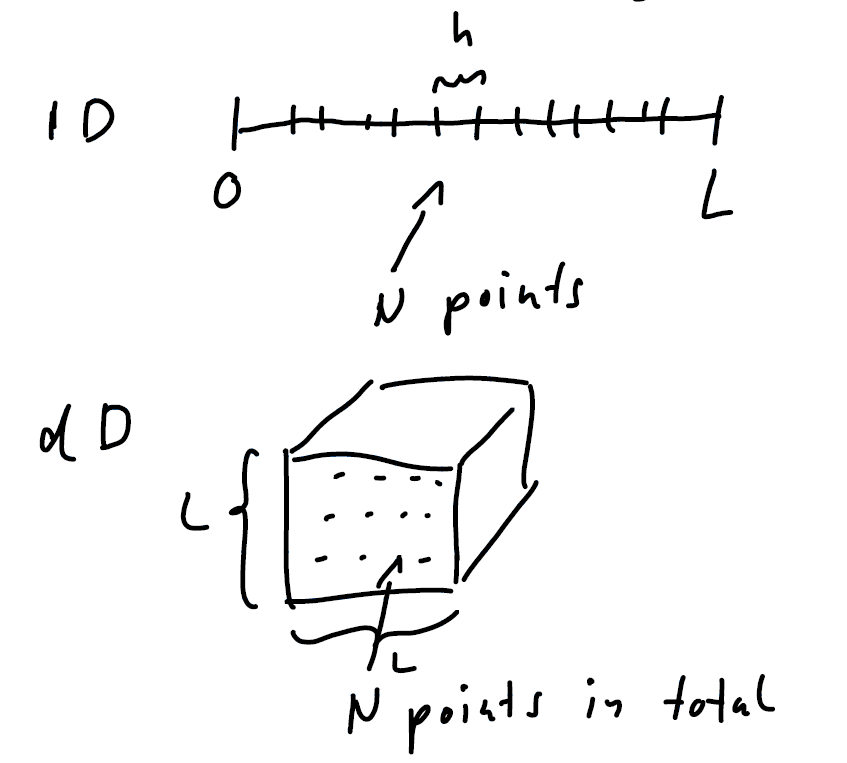Now, we perform numerical integration in $d$ dimensions using the same N amount of d-dimensional sections. The error will behave like: $$\sim h^k = (\frac{L}{N^{1/d}})^k\sim \frac{1}{N^{k/d}}$$ In the previous section, we have established that Monte Carlo integration has an error $\sim \frac{1}{\sqrt{N}}$. This means that Monte Carlo has smaller errors when $d>2k$. For integrating a Hamiltonian with many degrees of freedom, this condition is met very quickly.

Now that I have your attention, let's go to the really interesting part.

The need for importance sampling

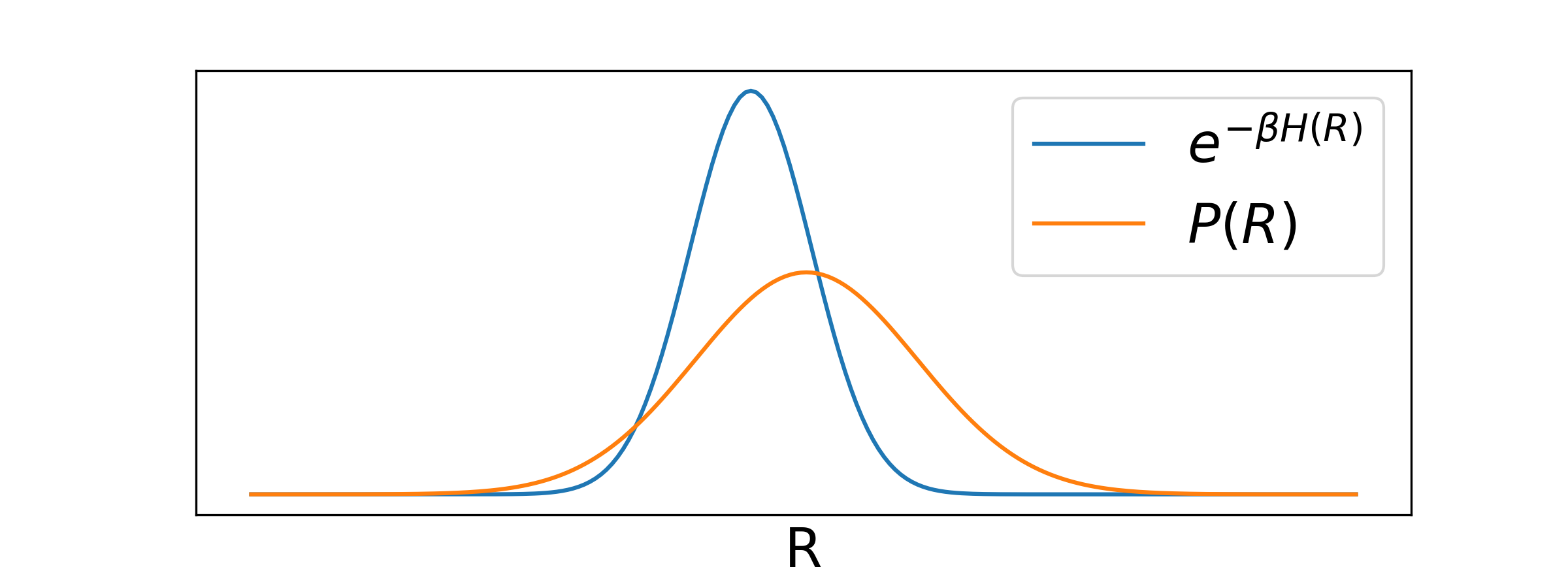
We could thus use Monte Carlo integration to evaluate $$\langle A\rangle = 1/Z \int e^{-\beta H(R)} A(R)dR$$ sampling uniformly over the configuration space described by $R$. However, this wouldn't be very efficient typically: In this intgral we have the Boltzmann factor that is non-zero only in a small region of configuration space (only a small region is physically relevant), as shown schematically in the sketch below:

Sampling unformily will in most cases sample an irrelevant configuration. Note that also in this case we would be guaranteed that the error of integrations drops like $1/\sqrt{N}$ int the limit of $N\rightarrow infty$ - but we will never practically reach it.

From Eq. (2) we see that we so not need to sample uniformly. Instead, we should be sampling from a random probability distribution that is concentrated in the physically relevant space. This is called importance sampling. In the following we will discuss two different approaches to importance sampling.

Approximate importance sampling

Sampling almost the right probability distribution

Let us consider the general case of computing the expectation value of a function $A(R)$ for a random variable distributed according to $p_\text{real}(R)$. (In the previous example, $p_\text{real}(R) = e^{-\beta H(R)}/Z$. We consider the general case here.) We then have to calculate the integral $$\int p_\text{real}(R) A(R) dR\,.$$ Ideally, we would now generate random variables $R_i$ that are distributed according to $p_\text{real}(R)$. However, this may be impractical. In this case we could instead try to sample from a nearby distribution $p_\text{sample}(R)$: In this way we can make sure to approximately focus on the physically relevant configurations.

Doing this requires us to rewrite the integral as $$\begin{eqnarray} \int p_\text{real}(R) A(R) dR = & \int p_\text{sample}(R) \underbrace{\frac{p_\text{real}(R)}{p_\text{sample}(R)}}_{=w(R)} A(R) dR\\ = & \int p_\text{sample}(R) w(R) A(R) dR\\ \approx & \frac{1}{N} \sum_{i=1}^N w(R_i) A(R_i) \tag{3} \end{eqnarray}$$ where the configurations $R_i$ are now sampled from $p_\text{sample}(R)$. When using this approximate probability distribution we thus have to introduce weights $w(R)$ into the average.

Why approximate importance sampling eventually fails

Approximate importance sampling is an attractive way of sampling: if we have a convenient and computationally efficient $p_\text{sample}$ we can apply the Monte Carlo integration and seemingly focus on the relevant part of the configuration space.

Unfortunatley, this approach becomes increasingly worse as the dimension of the configuration space increases. This is related to the the very conter-intuitive fact thatin high-dimensional space "all the volume is near the surface". This defies our intuition that is trained on dimensions $\leq 3$.

Let us look at a simple example. Consider two hybercubes in $d$ dimensions. The two hybercubes have side lengths $L$, so their volume is $L^d$. We now consider that the two hypercubes are shifted slightly with respect to each other, such that their overlap in every Cartesian coordinate direction is $\varepsilon L$ with $\varepsilon < 1$, as schematically sketched in 2D below:

We can now compute the ratio of the overlap volume to the volume of the hybercubes and find $$\frac{(\varepsilon L)^d}{L^d} = \varepsilon^d \xrightarrow{d\rightarrow \infty} 0!$$ So even for a slight shift, the overlap ratio will decrease exponentially with dimension.

This is also a problem when we sample with only a nearby probability distribution function. As the dimensionality of the configuration space increases, the overlap between the actual and the nearby probability distributions vanishes, and we keep on mostly sampling uninteresting space.

This effect directly shows in the weights. Let us demonstrate this using a simple example. Consider the case where $$p_\text{real}(x_1, \dots, x_d) = (2 \pi \sigma_\text{real})^{d/2} e^{-\frac{\sum_{k=1}^d x_k^2}{2\sigma_\text{real}}}$$ is a normal distribution with standard deviation $\sigma_\text{real}$. For the sampling distribution we use also a normal distribution, but with a slightly differen standard deviation $\sigma_\text{sample}$: $$p_\text{sample}(x_1, \dots, x_d) = (2 \pi \sigma_\text{sample})^{d/2} e^{-\frac{\sum_{k=1}^d x_k^2}{2\sigma_\text{sample}}}\,.$$ We will now compute how the weights $p_\text{real}/p_\text{sample}$ are distributed for different dimensionality $d$. In the example below we have chosen $\sigma_\text{real} = 1$ and $\sigma_\text{sample} = 0.9$ and sampling over $N=10000$ configurations: We see that as dimensionality increses, the distribution of weights gets more and more skewed towards 0. For a large dimensionality, almost all weights are very close 0! This means that most configurations will give little contribution to the weighted average in Eq. (3). In fact, this weighted average will be determined by the very few configurations that were by close to $p_\text{real}(R)$, end we end up with few physically relevant configurations again.

So in high-dimensional configuration space approximate importance sampling will eventually break down. The only way out is to sample even closer to $p_\text{real}(R)$. The ideal case would be to sample exactly from $p_\text{real}(R)$!

Metropolis Monte Carlo

Markov chain Monte Carlo

This leaves us a practical question: Can we sample exactly from an arbitrary $p(R)$? The answer is, maybe surprisingly, yes, and lies in using Markov chains.

So what is a Markov chain? Consider a sequence of random states $\{R_i\} = R_1, R_2, ..., R_N$. We say that the probability of choosing a new random state $R_{i+1}$ only depends on $R_i$, not any other previous states. Now, one can transition from one state to the other with a certain probability, which we denote as: $T(R \rightarrow R^\prime)$. This rate is normalised: $\sum_{R^\prime}T(R \rightarrow R^\prime)=1$. This simply means: you have to go to some state.

We can then write a rate equation to see what the chance is of obtaining state $p(R)$ at step $i+1$: $$p(R, i+1) = p(R, i) - \sum_{R^\prime}p(R, i)T(R \rightarrow R^\prime) + \sum_{R^\prime}p(R^\prime, i)T(R^\prime \rightarrow R)$$

But we want this Markov chain to eventually sample our probability distribution $p(R)$. This means that we want the probability to be stationary, such that we always sample the same distribution: $$p(R, i+1)=p(R, i)=p(R)$$ This simplifies the rate equation to: $$\sum_{R^\prime}p(R)T(R \rightarrow R^\prime) = \sum_{R^\prime}p(R^\prime)T(R^\prime \rightarrow R)$$ There are different ways for solving this equation. It is for sure solved by $$p(R)T(R \rightarrow R^\prime) = p(R^\prime)T(R^\prime \rightarrow R)$$ This particular solution of the rate equation is called detailed balance.

We can thus generate a desired probability distribution $p(R)$ by choosing the right $T(R^\prime \rightarrow R)$. This leads to the question: how do we generate the $T$ terms to get the correct probability distribution? The Metropolis algorithm solves this problem!

The Metropolis algorithm uses the following ansatz: $T(R \rightarrow R^\prime) = \omega_{RR^\prime} \cdot A_{RR^\prime}$. Here, the generation of the new state in the Markov chain is split into two phases. First, starting from the previous state $R = R_i$, we generate a candidate state $R^\prime$ with probability $\omega_{XX^\prime}$. This is the so-called "trial move". We then accept this trial move with probability $A_{RR^\prime}$, i.e. set $R_{i+1} = R'$. If we don't accept it, we take the old state again, $R_{i+1} = R$. Altogether, the probability of going to a state new state ($T(R^\prime \rightarrow R)$) is the product of proposing it ($\omega_{RR^\prime}$) and accepting it ($A_{RR^\prime})$.

The problem can we further simplified by demanding that $\omega_{RR^\prime}=\omega_{R^\prime R}$ - the trial move should have a symmetric probability of going from $R$ to $R^\prime$ and vice versa. The detailed balance equation then reduces to: $$\frac{A_{R^\prime R}}{A_{RR^\prime}} = \frac{p(R)}{p(R^\prime)} \tag{4}$$ Metropolis \emph{et al.} solved this as: $$A_{RR^\prime}=\begin{cases}&1 &\text{if} \ p(R^\prime) > p(R)\\ \\ &\frac{p(R)}{p(R^\prime)} &\text{if} \ p(R^\prime) < p(R)\end{cases}.\tag{5}$$ The key to understanding why Eq. (5) solves (4) is by observing that $A_{RR'}$ and $A{R'R}$ will necessarily be given by different cases in the Eq. (5).

Summary of Metropolis algorithm

1. Start with a state $R_i$
2. Generate a state $R'$ from $R_i$ (such that $\omega_{R_i,X'}=\omega_{R',R_i}$)
3. If $p(R') > p(R_i)$, set $R_{i+1}=R'$
   If $p(R') < p(R_i)$, set $R_{i+1}=R'$ with probability $\frac{p(R')}{p(R)}$
   else set $R_{i+1} = R_i$.
4. Continue with 2.

What determines the quality of the Metropolis sampling?

With the Metropolis algorithm we have a general procedure to sample according to any arbitrary probability distribution $p(R)$. In fact, the procedure works for any kind of arbitrary trial move (as long as the probabilities are symmetric) - we never detailed the move. It seems that Metropolis is pure magic!

What we need to realize is that we pay for the generality of the Metropolis algorithm with correlation. In fact, the degree of correlation is determined by the trial moves. A useful measure to determine the usefulness of a trial move is the acceptance ratio $\alpha=\frac{\text{number of accepted moves}}{\text{number of total moves}}$.

Let us demonstrate this using a simple example, and use the Metropolis algorithm to generate a Markov chain that samples a normal distribution $p(x) = (2 \pi \sigma)^{1/2} e^{-x^2/2\sigma}$. In this case, our configuration space is simply the real axis. As a trial move, we can randomly move a distance $d$ away from the original point: $$x' = x + d \times \text{random number between -1 and 1}$$ This trial move has symmetric probability for every distance $d$. Still, the choice of $d$ determines very strongly the correlation of the Markov chain as demonstrated below (for these simulation we used $\sigma=0$ and 200 Markov steps): In these pictures the probability distribution $p(x)$ is indicated by the shades of grey. The values in the Markov chain are plotted in blue.

When choosing a too large value of $d$ (left picture) we easily "overshoot" and land in a regin with low probability. Hence, the resulting acceptance ratio is small. But this leads to the Markov chain containing many repeated values as we keep on using the old value if the move is rejected! This leads to strong correlation and we sample effectively little independent data points.

When the value of $d$ is chosen too small (right picture) every move changes little about the configuration. As a consequence, the acceptance ratio is very large, but the speed which with we sample the configuration space is very slow. In fact, as seen above in this case only a part of the probability distribution is really sampled.

It is thus important to design the trial move in order to reduce correlation. In the example, this happens at some intermediate value of $d$. In many cases, such as here, the rule of thumb is that an acceptance ratio $\alpha \approx 1/2$ is a good target. But this depends on many aspects of the system.

In the end, the success of the Metropolis algorithm critically hinges on designing a good trial move.

Calculating the error of a mean computed using the Metropolis algorithm

The Metropolis algorithm generates correlated data $\{R_1, R_2, \dots, R_N\}$. As in the molecular dynamics project, we can use this data to estimate the mean, but when calculating the error of the mean it is essential to account for the correlations.

Which method is better?

The Metropolis algorithm has developed into one of the most important tools for importance sampling. Yet, it is not per se the superior method. As we saw, success of the Metropolis algorithm depends on designing a good trial step. This may not be easy for all situations. In addition, Metropolis necessarily generates correlated random numbers - compared to approximate importance sampling that can generate independent random configurations. Hence, the choice of method really depends on the problem at hand, and is in the end more a practical question of how well a method can be applied to a specific case.

This is also reflected in the three different project choices you have in for the second project. Two of them use the Metropolis algorithm (the simulation of the Ising model and the variational quantum Monte Carlo simulation), whereas the third uses approximate importance sampling (simulating polymers).